Google DeepMind’s TIPS v2 is a single model that can tell you what is in an image, where it is, and how it matches to text in one pass. It fuses a spatially aware image encoder with a text encoder so both image and text are mapped into the same embedding space, which makes zero-shot classification, image text retrieval, segmentation, and depth estimation possible without any fine-tuning. The model is small, under 1 GB, and can run on CPU, yet it brings global understanding, spatial detail, and text alignment together.
To run it locally on Ubuntu, set up a Python virtual environment, launch Jupyter, download and load the model, preprocess images to 448 by 448, then encode images and texts to compute similarities. The image encoder outputs a single global vector for the whole image and a grid of patch vectors that carry position-aware meaning, which you can visualize or feed into simple heads for masks and depth. With the same embeddings, you can ask open label questions like is this a cat or a Siamese cat and get reliable zero-shot predictions.
What this model does
Most image AI models are good at one thing. CLIP models can match images to text but have no idea about spatial layout, and self-supervised vision models like DINOv2 understand spatial detail really well but cannot process text.
TIPS combines both worlds. One model, zero-shot classification, segmentation, depth estimation, no fine-tuning.
TIPS has two encoders, an image encoder and a text encoder. You feed it an image and a text description, both get converted into numerical representations or embeddings, and they live in the same shared space.
Because the image encoder is spatially aware, the embeddings carry where things are, not just what things are.
You can do zero-shot classification by asking is this a cat or a Siamese cat without any training. You can do image text retrieval by comparing text embeddings to the image embedding.
Because the spatial features are rich and nuanced, you can also do segmentation and depth prediction with the same backbone.
Read More: Run a local model end to end
How the embeddings are structured
The image encoder emits a classification token and patch tokens.
CLS, the classification token, is the model’s single global summary of the entire image packed into 1 by 768 dimensions. Patch tokens have shape 1 by 1024 by 768 for a 32 by 32 grid, which means the model cut the image into 1024 small patches and gave each patch its own 768 number description.
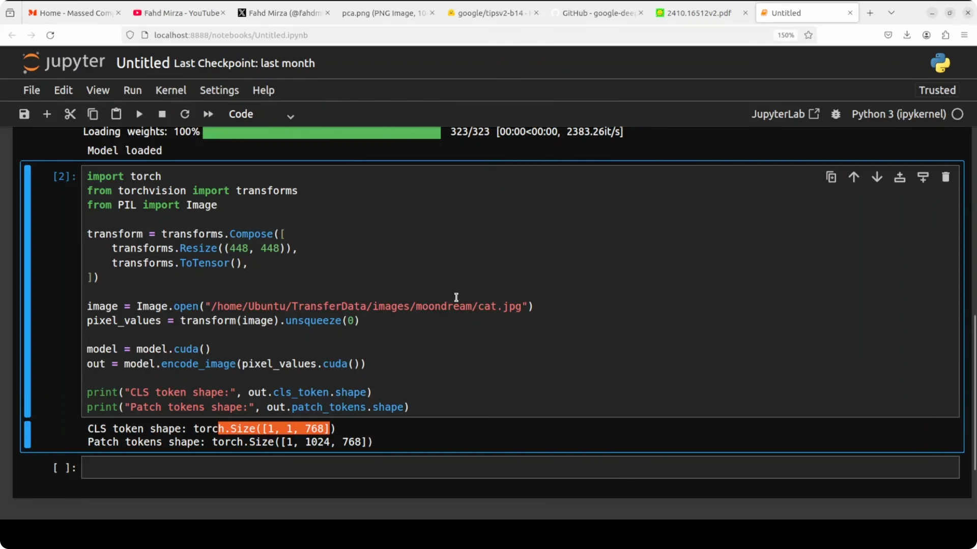
It does not just know there is an object. It knows where the object is and where other components of the image are, like the bed or the lamp in a typical indoor scene.
That spatial awareness is what makes TIPS different from single purpose models.
Why spatial signals matter
Inside the latent space, those 1024 patches naturally cluster into foreground and background. Regions that belong together tend to move together in embedding space even without explicit labels.
Different regions, different signals, different meanings, learned from images and text during pre-training.
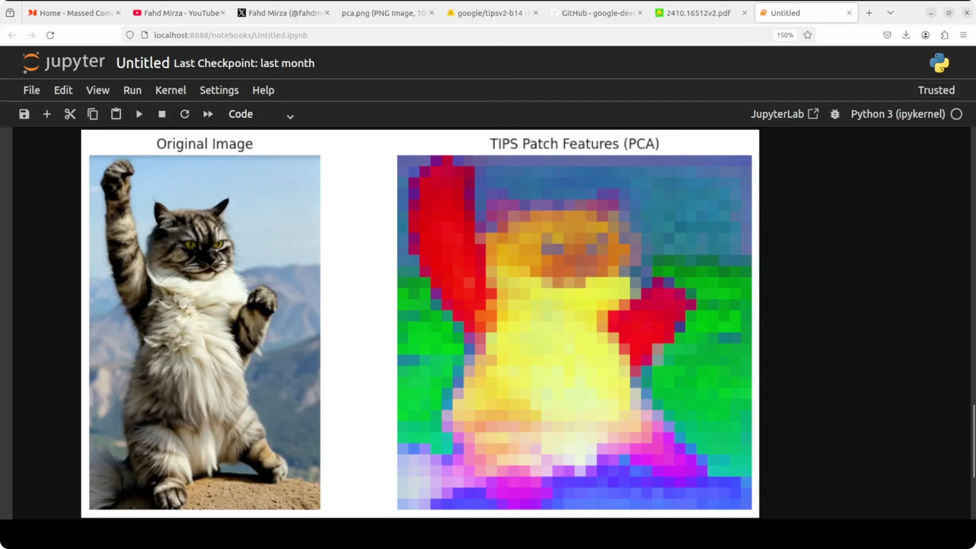
This is spatial awareness in action that you can project for masks or depth without teaching a new network from scratch. The same backbone supports global understanding and per region reasoning.
One model, all of that.
Read More: See tips on handling AI subscription quotas
Run it locally
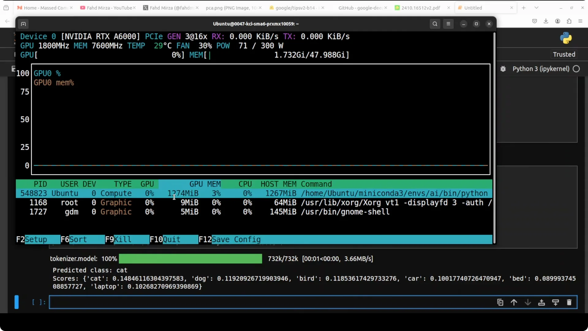
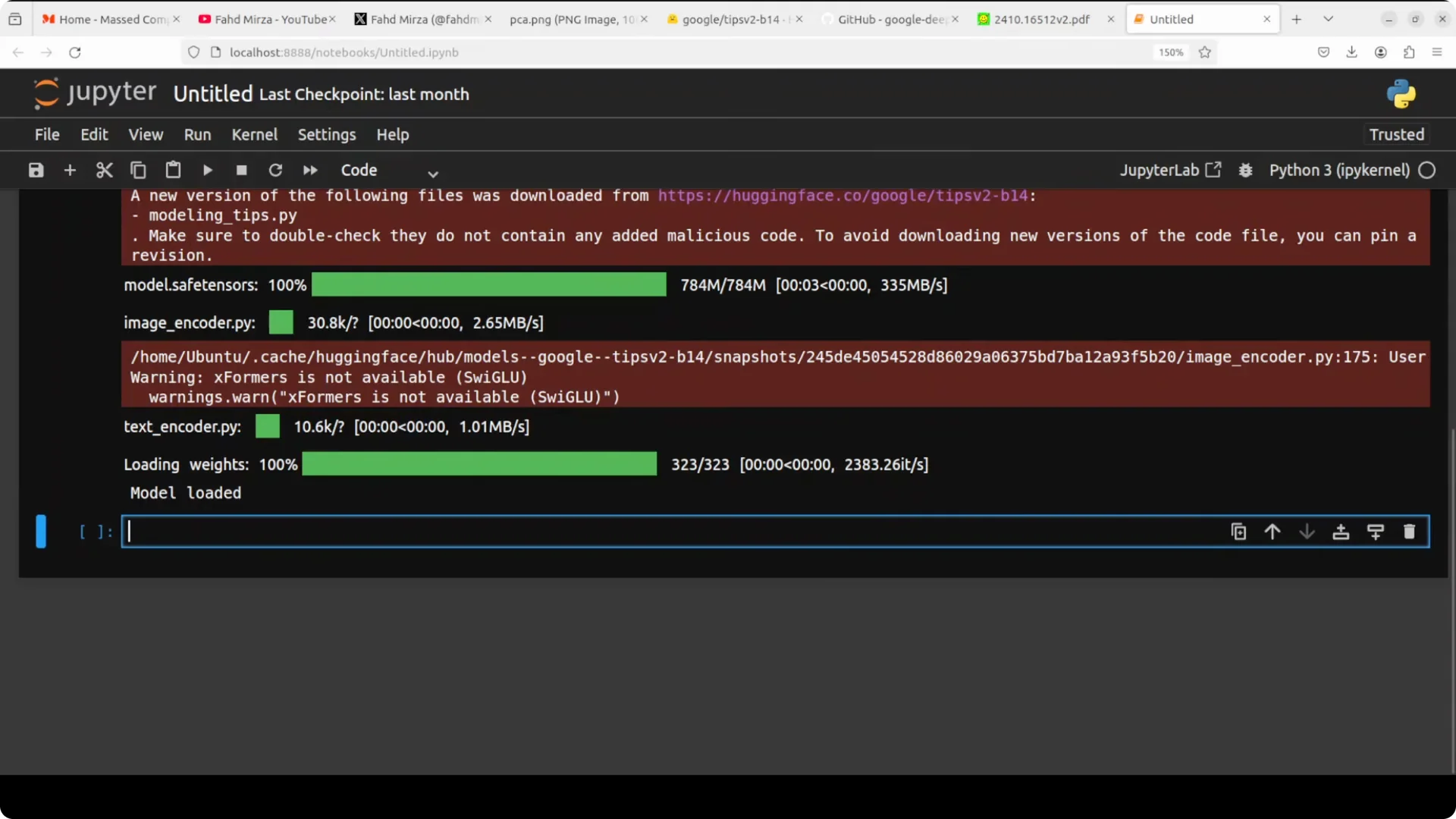
I used Ubuntu with an Nvidia RTX A6000 with 48 GB of VRAM, but you can run on CPU for small batches. The model footprint is under 1 GB and inference is quick even without a GPU.
VRAM usage can remain minimal until you push large batches or high resolution.
Step 1. Create and activate a virtual environment.
python3 -m venv .venv
source .venv/bin/activate
Step 2. Install Jupyter and your preferred deep learning stack. Match your Torch build to your system and CUDA if you plan to use a GPU.
pip install jupyter
Step 3. Launch Jupyter.
jupyter notebook
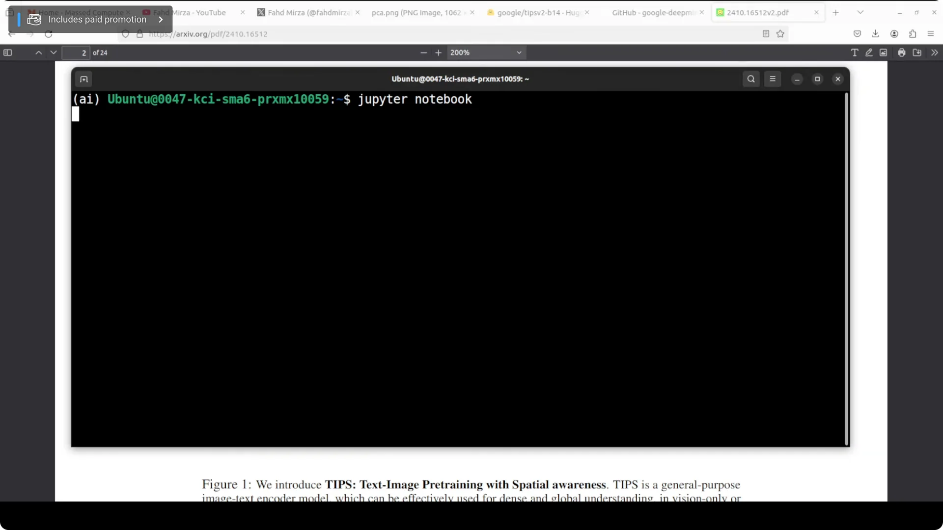
Step 4. Download and load the model weights using the project’s loader. Keep the model on CPU if you want the lowest memory footprint.
Step 5. Preprocess images to 448 by 448 before encoding. Center crop or resize consistently so the patch grid aligns.
from PIL import Image
img = Image.open("your_image.jpg").convert("RGB")
img = img.resize((448, 448))
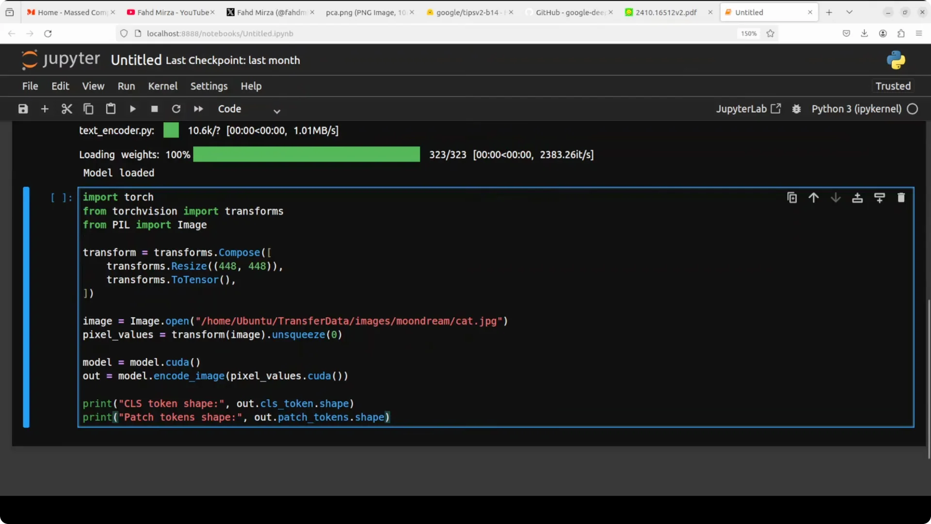
Step 6. Run the image through the TIPS image encoder to get the CLS vector and the patch token grid. Step 7. Encode candidate texts, compare similarities to the image embedding for zero-shot classification and retrieval, and project patch tokens if you want segmentation or depth outputs.
To keep an eye on GPU memory during experimentation, run:
nvidia-smi
Read More: Quota workarounds and usage planning
Zero-shot classification
Zero-shot classification here means you pass an image and a list of label strings and the model tells you what matches what.
The score is a similarity value, so the label with the highest similarity to the image embedding wins. No training, no fine-tuning.
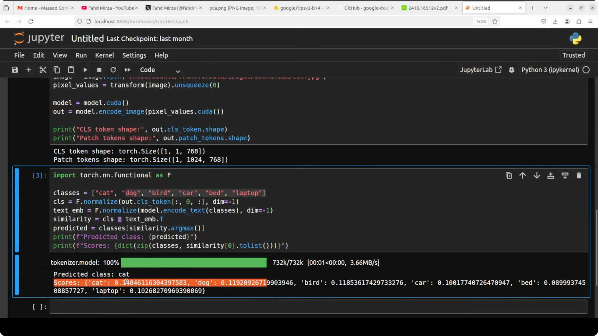
You can extend this by passing hierarchical labels to get coarse to fine classification in a single pass. You can also threshold similarities to reject unknowns.
This makes quick pilots practical without data collection.
Image text retrieval
Encode text prompts and compare them against the image embedding. The closest text in embedding space surfaces as the most relevant caption or description.
This is the same mechanism that powers open label search over image collections.
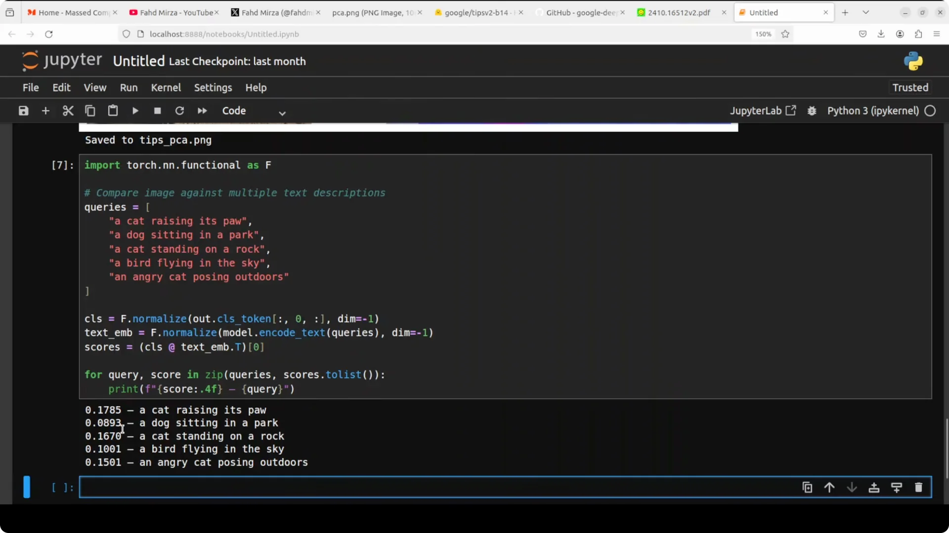
Retrieval scales naturally because you can precompute image embeddings and store them in a vector index. At query time you only encode text and do a nearest neighbor search.
Latency stays low and accuracy is robust because the space is shared.
Read More: If your account access gets restricted, start here
Segmentation and depth
Because patch tokens encode where things are, you can visualize regions or build lightweight heads that map patch embeddings into masks. Even a simple projection with a small decoder can yield clean segmentation for prominent subjects.
The same patch grid supports depth prediction with a shallow regression head.
Tasks that normally need completely different models can share this single encoder. You avoid shuttling data across multiple backbones and keep deployment simple.
Global understanding and spatial detail live in one stack.
Hardware notes
The model download is lightweight at about 784 megabytes. Inference runs on CPU, with GPU optional for throughput or larger batches.
Keep batch sizes small on CPU for quick iteration.
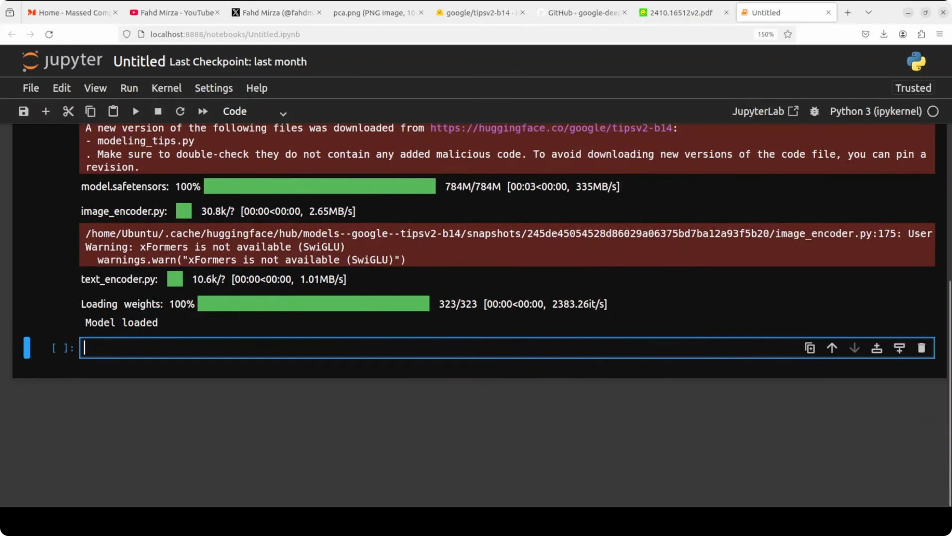
If you hit network or proxy errors while fetching dependencies, fix them before retrying the notebook.
HTTP errors from corporate networks are common during package installs.
Read More: Troubleshoot HTTP 500 and related setup errors
Practical use cases
Search and organize large photo libraries by open ended text queries. Enrich product catalogs with zero-shot tags and location cues for backgrounds and foregrounds.
Power visual chat or agent pipelines that need both global labels and per region features.
Do visual grounding for robotics by mapping text instructions to regions in view. Speed up dataset curation by prefiltering candidates for labeling.
Prototype depth aware AR effects from a single encoder.
Read More: Manage usage limits while experimenting
Final thoughts
You just saw what makes this model special.
One encoder pair handles global understanding, spatial understanding, and text alignment, all in one. Bigger variants are available if you need more capacity, while the small one already brings strong results under tight resource budgets.